4.3.1
Managing Assets Using Condition Based Management
The condition-based management is the most complex of the approaches introduced in Section 4.2 and requires a commitment to the collection of reliable inventory and condition information over an extended period and the of condition models to predict future deterioration to evaluate the type and timing of various treatment actions in terms of risk and performance.
Using Computerized Management Systems to Optimize Life Cycle Management
For condition-based analysis, computerized management systems are valuable tools for evaluating life cycle strategies. Computerized systems support the larger life cycle management process by providing relevant, reliable information and analysis results to decision makers at the right time.
Condition-based management is common for pavement and bridge assets. Often pavement and bridge decision making is supported by a computerized system that is used to support optimized life cycle management. The results from this analysis provide insights into optimal life cycle strategies for all network assets or for a specific group of assets. These models can be configured to include the effects, maintenance, preservation, rehabilitation, and reconstruction actions. Depending on the type of condition-based modeling approach, uncertainty can also be included.
Various life cycle scenarios can be generated by modifying one or more variables in the analysis. By running multiple network-level scenarios and comparing the results, pavement and bridge management systems can identify viable life cycle strategies and help an agency select the strategy that best achieves the stated objectives.
More information on the use of pavement and bridge management systems is available in the FHWA document, Using a Life Cycle Planning Process to Support Asset Management: A Handbook on Putting the Federal Guidance into Practice. Life cycle planning is a required component of risk-based TAMPs developed by state DOTs (23 CFR 515), that uses computerized asset management systems to establish long-term life cycle strategies for pavements, bridges and other highway assets. NCHRP Report 866, Return on Investment in Transportation Asset Management Systems and Practices, provides an assessment of how state DOTs have implemented asset management systems, including practice examples. The end of this section includes a how-to guide for using a pavement management system for life cycle planning, a requirement for risk-based TAMPs developed by state DOT’s for pavements and bridges on the National Highway System (23 CFR 515).
These computerized systems are designed to develop network-level scenarios for analyzing the impacts of different program variables over long periods of time. Typical pavement management scenarios will cover 10 to 40 years, while bridge management scenarios may need to cover 100 years or more to ensure inclusion of multiple life cycles within the scenario.
Various life cycle scenarios can be generated by modifying one or more variables in the analysis. By running multiple network-level scenarios and comparing results, pavement and bridge management systems can identify viable life cycle strategies and help an agency select a strategy that best achieves the stated objectives.
Ohio DOT
As required under MAP-21, Ohio DOT conducted a risk assessment to identify the most significant threats and opportunities to its pavements and bridges. The analysis revealed that anticipated flat revenues, combined with the annual increases in cost to pave roads and replace bridges, would lead to significant reduction in conditions without changes to existing practice. The potential deterioration in pavement and bridge conditions were expected to significantly increase future investment needs due to the increase in substantial repairs that would be required.
Following the risk assessment, a life cycle analysis was conducted. The analysis found that by focusing on the increased use of chip seals and other preventive maintenance treatments on portions of the pavement network, the annual cost of maintaining the network could be reduced. A life cycle analysis for bridges showed similar results. The bridge analysis found that with just 5 percent of the NHS bridges receiving a preservation treatment annually, the DOT could reallocate $50 million each year to other priorities. The investment strategies outlined in the TAMP and the changes made to the DOT’s existing business processes enabled the agency to offset the potential negative impact of the anticipated flattened revenue projections.
The differences in the adopted life cycle strategies are compared to the past strategies in the Figure. Although the total number of treatments applied over the analysis period increases, the annual life cycle cost decreases because of the reduction in the number of rehabilitation strategies needed.
Ohio DOT’s Pavement Preservation Strategy Comparisons
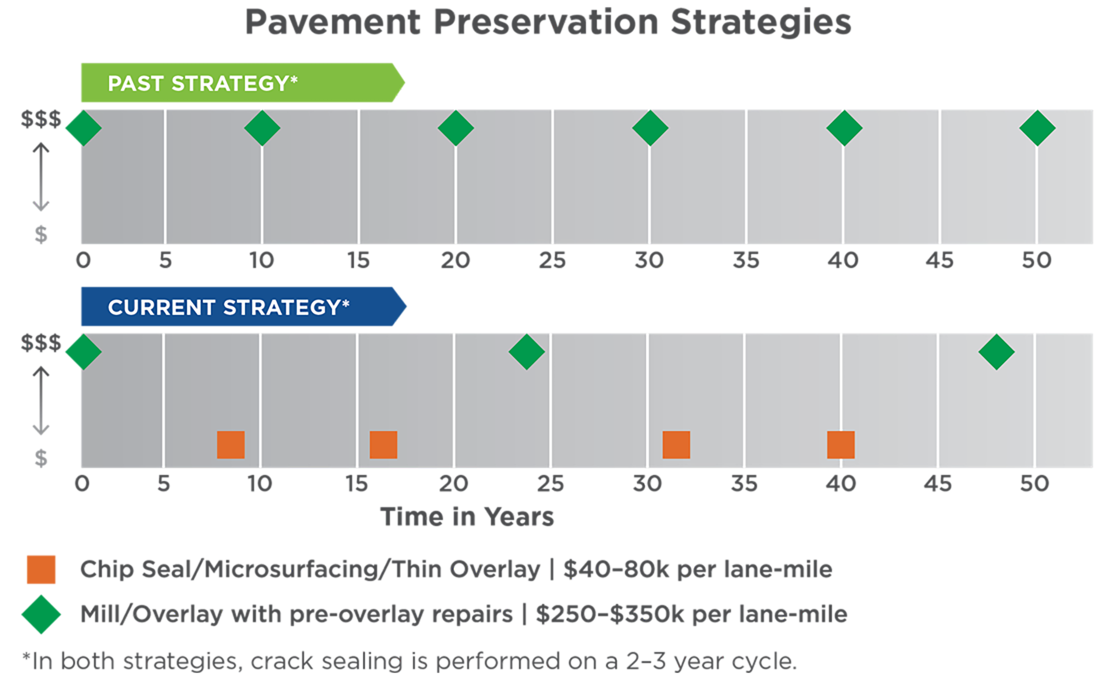
Source: Ohio DOT Transportation Asset Management Plan. 2018. http://www.dot.state.oh.us/AssetManagement/Documents/ODOT_TAMP.pdf
Minnesota DOT
In its 2019 Transportation Asset Management Plan (TAMP), MnDOT went beyond the scope of pavements and bridges as mandated by 23 CFR Part 515, addressing a comprehensive range of assets, including culverts, deep stormwater tunnels, overhead sign structures, high-mast light tower structures, noise walls, traffic signals, lighting, pedestrian infrastructure, buildings, and intelligent transportation system (ITS) components. MnDOT established expert work groups for each asset class to assess data availability, risks, mitigation strategies, measures, targets, and investment strategies. The Transportation Asset Management System (TAMS) was developed to manage asset inventory, condition data, and capture maintenance resources. TAMS integrates asset data, historical expenditures, and decision trees for culvert maintenance, facilitating life-cycle analysis, maintenance demand estimates, and performance evaluation. While traffic signals and ITS assets are being analyzed within TAMS, building management and sidewalk data are stored in separate databases.
Predicting Asset Performance
TAM Webinar #26 - Asset Inventory Condition, Target Setting, and Ten Year Projections
A life cycle strategy is enhanced by the availability of models and analysis tools that facilitate the evaluation of different combinations of treatment type and timing across the asset class. For this analysis a model that predicts future asset deterioration and response to treatments is required.
For condition-based approaches to managing assets, historical performance is typically used as a baseline for developing models to predict future performance. The predicted conditions are used to determine the type of treatments that may be needed over an asset’s service life, so the ability to accurately predict asset conditions in the future, with and without treatment, is an essential component of asset management. Models are developed by comparing performance, typically measured as asset condition, over time with actions or treatments performed on specific assets. This means that performance is associated to the last action or treatment that impacted performance in a positive way. However, assets may also receive treatments that delay the onset or advancement of distress. As a result, most models assume assets receive some level of preventive or routine maintenance between more significant treatments. If agency practices change to delay or cease maintenance activities, assets may not perform as models predict.
Several methods can be used to estimate future asset performance, the two most
common of which, deterministic and probabilistic, are described below. Additional information has been published by NCHRP (Report 713, 2012 ): Estimating Life Expectancies of Highway Assets. This report also contains guidance on selecting the most appropriate modeling approach for various highway asset classes.
Deterministic Modeling
Deterministic modeling is a common and relatively simple approach for using historic data to predict future asset performance. Deterministic models apply regression analysis to one or more independent variables, typically condition over time, and develop a “best-fit” equation to determine the rate at which asset conditions change. The independent variables are used to predict a single dependent variable, most commonly represented as the predicted condition at some point in time in asset management applications. Developing deterministic models is relatively easy but relies on quality data collected consistently over several years to produce dependable results. Deterministic models are more easily implemented as they are more readily paired with linear program solving. They also provide consistent outputs. The downside of deterministic models is the limited insight that they provide into the cost uncertainty surrounding a strategy.
Probabilistic Modeling
Unlike deterministic models, which provide a single repeatable outcome, probabilistic models provide a distribution of possible strategies that provides insight into the cost uncertainty of plans. Probabilistic models can also more readily accept uncertainty in other variables, as represented by the shading in Figure 4.7. Given that condition changes are probabilistic, no two strategies that the model will provide are the same. This means that multiple iterations of the model with the same inputs can provide different results. Accordingly, probabilistic models are useful for setting funding limit expectations, while deterministic models help to provide insights into which projects are best to apply to specific assets.
Common approaches to developing probabilistic models are the Markov, Semi-Markov and Weibull models. Markov modeling works well for assets with condition ratings based on regular inspections. There are several ways of establishing a Markov model, but the simplest is to calculate the proportion of assets that change from one condition state to the next in any given year. These proportions are then used to develop what is known as the transition matrix. At the start of the model run, an asset “knows” its condition state. Once this is known there is then a probability it will change from its current condition state to the next in any given year. While these types of Markov approaches have been widely used, they do not necessarily model deterioration effectively, as the rate of change of condition increases with time. To address this, Semi-Markov models are used. Like Markov, Semi-Markov models have a condition transition matrix, but this is also augmented with a time selection matrix. In these models the probability of a condition jump is calculated, then the length of time an asset will remain in that condition state is also selected. Using more advanced mathematical techniques, the Semi-Markov approach can be expressed similarly to the Markov approach, but for Semi-Markov, the transition matrix changes with time. This reflects the increasing likelihood the asset will transition (deteriorate faster as its ages). Such models are typically used on long-lived assets.
A Weibull model offers another approach for modeling asset deterioration. A Weibull distribution predicts the likelihood of asset failure or deterioration as a function of age. Weibull models are particularly useful for addressing assets rated on a pass/fail basis during inspection. The Weibull model provides an additional factor meant to address the increasing or decreasing likelihood of an asset moving from an acceptable to an unacceptable state between inspection cycles. Reliability is the inverse of the probability of failure (i.e. 1 -p(f)). Reliability, like Weibull can thus be used to assess the likelihood an asset will provide the required service. The relationship between time and reliability is assessed by analyzing asset behavior to understand potential modes of failure. This analysis is a core aspect of reliability-centered maintenance, and is more typically used on short lived assets.
Figure 4.7 Example of a Probabilistic Model
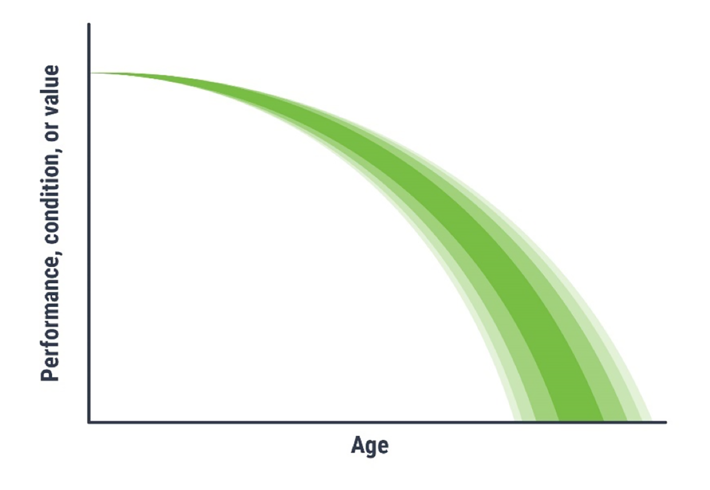
Source: Adapted from Transportation Research Board. 2012. Estimating Life Expectancies of Highway Assets, Volume 1: Guidebook. https://doi.org/10.17226/22782.
Accounting for Uncertainty in Asset Performance
Performance modeling uses historic data to estimate future performance; however, not all future events are predictable nor is past performance necessarily a predictor of future performance. This section considers the how uncertainty can be introduced into the analysis.
The unpredictability of future events introduces uncertainty into prediction models. Additionally, the amount of uncertainty tends to increase with time so their affects are compounded. As outlined in the previous section, probabilistic modeling is one approach that can be used for accounting for uncertainty, but what level of uncertainty is acceptable?
To minimize uncertainty, an agency must first understand the source of the uncertainty. A common type of uncertainty related to asset management is the behavior of the assets themselves. Due to the advancement of technology and knowledge and differences in materials and construction practices, there can be significant differences in performance between otherwise similar assets. The change in behavior can be positive, such as the introduction of epoxy-coated reinforced steel in bridge decks to delay the onset of corrosion from road salt intrusion or the introduction of Superpave and performance graded asphalt binders to reduce pavement cracking and rutting. Other changes in behavior are less easy to predict, such as the impact of salt intrusion on prestressed, post-tensioned concrete box-beam bridges. Other sources of uncertainty include:
- Weather events, e.g. flooding, drought, or freeze-thaw
- Earthquakes
- Climate change
- Traffic accidents
- Data inaccuracies
- Inaccurate models
- Poor assumptions
Uncertainty caused by variability in the data can often be addressed through the development of quality assurance plans that describe the actions an agency has established to ensure data quality, whether the data is collected in-house or by a contractor. Common quality assurance techniques include documented policies and procedures to establish data quality tolerance limits, independent reviews of collected data, and training of data collection crews. Data management strategies are discussed in more detail in Chapter 7.
To evaluate the accuracy of models and assumptions, agencies can include multiple scenarios in their life cycle planning analysis to test the impact of different decisions. This type of sensitivity analysis can be helpful in identifying areas in need of further research or developing contingency plans if the initial assumptions turn out to be inaccurate.
To understand whether time and effort should be invested in minimizing uncertainty, a risk-based approach can be used. Assuming the consequence arising from a defined issue or event remains the same, the cost in terms of data collection of reducing uncertainty can be investigated. As an example, the condition state of an asset, as determined using a visual approach, may not provide the required level of insight, which results in poor or unknowable treatment decisions. To minimize the uncertainty, extra testing can be carried out. The level of testing would be defined by the risk-cost reduction ratio. Similarly, with climate change, how much would have to be invested in studies to understand the effects on asset longevity? Thus, through risk management, an agency determines which risks are tolerable and which must be actively managed through investigations, studies other research. The risks are identified, prioritized, and tracked using a risk register (see Chapter 2). For those risks that should be managed, plans are developed to outline actions that will be taken to mitigate threats or take advantage of opportunities, as discussed in Chapter 6.
Halifax Regional Water Commission
Halifax Regional Water Commission (Halifax Water) has employed a deterministic modelling approach to create a plan for their storm water assets. The management system was used for long-term planning their culvert portfolio (approximately 1744 cross culverts on 3700 lane km of regional roads). The software uses deterioration curves, a temporal model periodic simulation model and has integrated Geographic Information System (GIS) capabilities.
Initially the analytical objective of the model was to maximize the average condition of all the culverts and minimize the investment. Several constraints were embedded within the initial model analysis including:
- Non-Increasing percentage of culverts in critical condition
- Replace all culverts that exceed expected useful life
- Budget not to exceed scenario
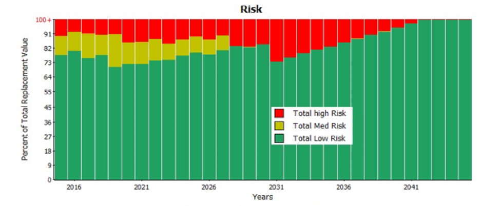
The scenario analysis allowed Halifax Water to establish a minimum investment level required to bring the portfolio to an acceptable average condition state, have a reliable forecast of future condition trends, and quantify an estimate of accepted risk of failures. The figure below shows the agency’s forecasted risk of failure over time based on the selected strategy and projected funding.
NBDTI forecasted culvert conditions using a deterministic model.